
12.3, 12.4 Linear Regression
Problem 1
For each problem, select the best response.
(a) The owner of a chain of supermarkets notices that there is a positive correlation between the sales of beer and the sales of ice cream over the course of the previous Seasons when sales of beer were above average, sales of ice cream also tended to be above average. Likewise, during seasons when sales of beer were below average, sales of ice cream also tended to be below average. Which of the following would be a valid conclusion from these facts?
- A scatterplot of monthly ice cream sales versus monthly beer sales would show that a straight line describes the pattern in the plot, but it would have to be a horizontal line.
- Sales records must be in error. There should be no association between beer and ice cream sales.
- The sale of beer and ice cream may both be affected by another variable such as the outside temperature.
- Evidently, for a significant proportion of customers of these supermarkets, drinking beer causes a desire for ice cream or eating ice cream causes a thirst for beer.
- None of the above.
(b) A researcher observes that, on average, the number of children in cities with major league baseball teams is larger than in cities without major league baseball teams. The most plausible explanation for this observed association is
- the high number of children is responsible for the presence of more major league baseball teams (more children means potentially more fans at the ballpark since people like to bring their kids to baseball games, thus making it attractive for an owner to relocate to such cities).
- the presence of a major league baseball team causes the number of children to rise (perhaps people decide to have children so they can bring them to the ballpark).
- the observed association is purely coincidental. It is implausible to believe the observed association could be anything other than accidental.
- the association is due to the presence of a lurking variable (major league teams tend to be in large cities with more people, hence a greater number of children).
- None of the above.
(c) When possible, the best way to establish that an observed association is the result of a cause-and-effect relation is by means of
- the correlation coefficient.
- a well designed experiment.
- the square of the correlation coefficient.
- the least squares regression line.
- None of the above.
Correct Answers
- C
- D
- B
Problem 2
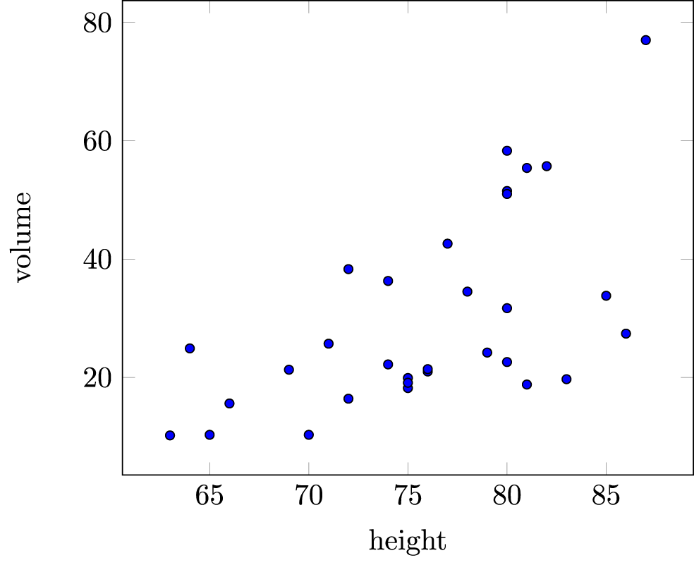
The height (in feet) and volume of usable lumber (in cubic feet) of 32 cherry trees are measured by a researcher. The goal is to determine if volume of usable lumber can be estimated from the height of a tree. The results are plotted below.
(a) In this study, the response variable is
- height.
- height or volume. It doesn’t matter which is considered the response.
- neither height nor volume. The measuring instrument used to measure height is the response variable.
- volume.
(b) The scatterplot suggests
- there is an outlier in the plot.
- there is a positive association between height and volume.
- both A and B.
- neither A nor B.
Now consider the following scatterplot of the weight of cars (in thousands of pounds) versus the miles they travel per gallon of gas consumed (mpg).
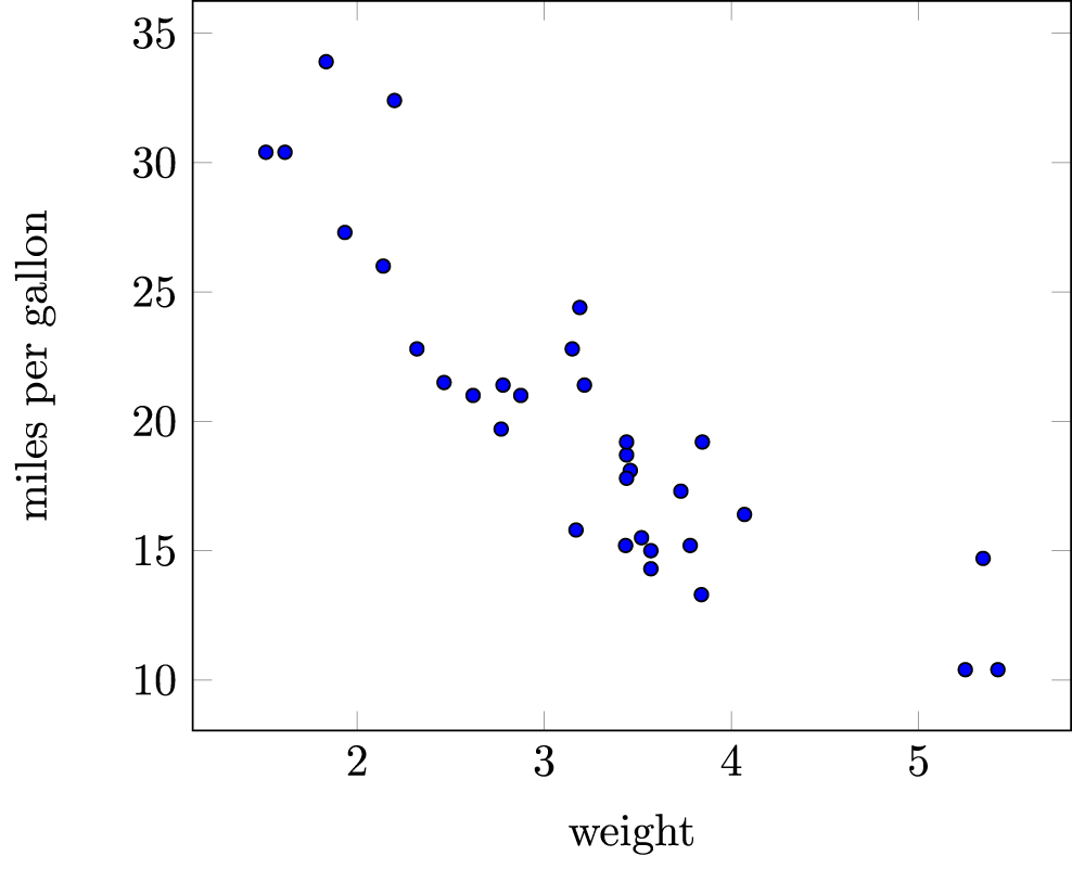
(a) A plausible value for the correlation between weight and mpg is
- -1.0
- +0.2
- -0.9
- +0.7
Correct Answers
- D
- C
- C
Problem 3
Match the correlation coefficients with their scatterplots. Select the letter of the scatterplot below which corresponds to the correlation coefficient.
A.

B.

C.

D.

- r = -0.66
- r = -0.99
- r = 0.70
- r = 0.99
Correct Answers
- r = 0.70
- r = -0.66
- r = -0.99
- r = 0.99
Problem 4
Data were collected from all 10 year olds in a soccer league. Based on this dataset, a least squares regression model was fitted to predict weight Y (in kg) from height X (in cm). The model fitted was
[latex]Y = 0.99X - 101.24[/latex]
The interpretation of the slope of the regression line would be
- For each 1 cm increase in height, you would expect the weight to increase by 0.99 kg
- For each 1 kg increase in weight, you would expect the height to decrease by 101.24 cm
- For each 1 kg increase in weight, you would expect the height to increase by 0.99 cm
- For each 1 cm increase in height, you would expect the weight to decrease by 101.24 kg
Correct Answers
A
Problem 5
Is the number of games won by a softball team in a season related to the team batting average? The table below shows the batting average (in thousandths) and the number of games won of 8 teams.
| Team | Batting Average | Games Won |
| 1 | 272 | 40 |
| 2 | 262 | 45 |
| 3 | 317 | 30 |
| 4 | 304 | 41 |
| 5 | 276 | 44 |
| 6 | 286 | 45 |
| 7 | 263 | 50 |
| 8 | 320 | 37 |
Using batting average as the explanatory variable x, do the following:
- The correlation coefficient is [latex]r =[/latex]
- The equation of the least squares line is [latex]\hat{y} =[/latex]
Correct Answers
- -0.815699
- -0.214446x + 103.073
