
3 Probability
Up until now, interpretations of data have pretty much come from “the seen”, or what can be observed. In this chapter, we will deal with the “unseen”, the unobserved, which are probabilities. Probability can be a difficult concept to grasp, yet we use it every day. We ask such questions as “What are the chances it is going to rain today?”, “How likely is it that this relationship will last?”, or “What is the chance that I will get an A out of this statistics class?”. We answer these questions with “fair chance”, “likely”, or “highly likely”. A pertinent question is, “How likely is it that you will learn about the two topics of statistics and social justice issues at the same time?” This question is for you to answer.
Learning Outcomes
There are many aspects of probabilities that will be covered in this chapter:
- The Definition of Probability in Statistics
- Rules of Probability
- Probability Distributions
- The Normal Curve as a Probability Distribution
- The Standard Normal Distribution
- Blending Probability with Social Justice Issues
Now, let’s begin our journey to understand this “mystical” concept.
3.1. Probability Definition in Statistics
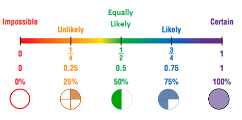
Simply put, probability means possibility—the extent to which something is likely to happen. As shown in Figure 1, probability (P) can range from 0 to 1, where 0 means the event is an uncertain (or impossible) one and 1 indicates a certain event. Probabilities of .05 or .10 imply very unlikely circumstances, and high probabilities such as .90, .95, or .99 signify very probable or likely outcomes.
Probability is also a mathematical tool to study randomness. A phenomenon is random if individual outcomes are uncertain. A random variable represents a value associated with each outcome of a probability experiment. For a random variable, x, the word random indicates that the value of x is determined by chance. The expected value of a random variable can be positive, negative, or zero.
A probability model is a mathematical description of a random phenomenon consisting of a sample space, S, which is the set of all possible outcomes. If S is the sample space in a probability model, the P(S)=1. A probability model with a finite sample space is called finite. Finite probability models are often called discrete probability models.
An event is an outcome or a set of outcomes of a random phenomenon; it is the subset of the sample space.
Now Try It Yourself
Elliott et al. (2006) created a hybrid method (geocoding and surname analyses) for estimating race/ethnicity and associated disparities where self-reported race/ethnicity data is unavailable. Geocoding uses an individual’s address to link individuals to census data about the geographic areas where they live. For example, knowing that a person lives in a Census Block Group (a small neighborhood of approximately 1,000 residents) where 90 percent of the residents are African American provides useful information for estimating that person’s race. Surname analysis infers race/ethnicity from surnames (last names). Insofar as a particular surname belongs almost exclusively to a particular group (as defined by race, ethnicity, or national origin), the researchers used well-formulated surname dictionaries to identify a probable membership in a group.
Problem #1: Verify whether the researchers’ findings in Table 1 below is a legitimate assignment of probabilities:
| Surname | Asian | Hispanic | African American | White/Other |
| Wang | .937 | .008 | .008 | .048 |
| Martinez | .010 | .845 | .021 | .125 |
| Jones | .061 | .022 | .129 | .787 |
Answer:
To be a legitimate probability distribution, the sum of the probabilities for all possible outcomes must equal to 1. For the surname (n=3), the probabilities are 1.00 for Wang, 1.00 for Martinez, and .999 for Jones. Of the surname group, only two have a legitimate probability distribution.
For the ethnic groups, the probabilities are 1.00 for Asian, .875 for Hispanic, .158 for African American, and .96 for White/Other. The Asian Group is the only ethnic group that has a legitimate assignment of probabilities.
Thus, of the seven outcomes, only three outcomes add up to 1 and have legitimate probability distributions.
3.2 Rules of Probability
Rule #1: The probability associated with an event is the number of times that event can occur relative to the total number of times any event can occur. This is known as the classical or theoretical probability. The empirical or statistical probability is based on observations obtained from probability experiments. The empirical probability of an event E is the relative frequency of event E.
Rule #2: The complement of event E is the set of all outcomes in a sample space that are not included in E and is denoted as E’, pronounced as E prime. The complement or converse rule of probability is 1 minus the probability of that event occurring.
P(E’) = 1 – P(E)
Based on the example in the box below, the recidivism rate in the United States is 77%. In other words, a person released from prison has a 77% probability of being rearrested. The converse is non-recidivism. The probability that a discharged inmate does not recidivate is 1 – .77 = .23.
Recidivism Rate:
Applying the Equity Lens
Rule #3: The addition rule of probability states that the probability of obtaining any one of several different and distinct outcomes equals the sum of their separate probabilities. The addition rule always assumes that the outcomes being considered are mutually exclusive or disjointed—that is, no two outcomes can occur simultaneously (Levin & Fox 2006)[2].
P (A or B or C) = P (A) + P (B) + P(C) Mutually exclusive events
P (A or B or C) = P (A) + P (B) + P(C) – P(A and B) – P(A and C) – P(B and C)
+ P (A and B and C)
Example of Adding Probabilities: Suppose that a defendant in the January 6th United States Capitol Attack has a .55 probability of being convicted as charged, a .26 probability of being convicted of a lesser degree, and a .19 chance of being found not guilty. The chance of a conviction on any charge is .55 + .26 = .81. Note also that this answer agrees with the converse rule by which the probability of being found not guilty is 1 – .19 = .81.
Now Try It Yourself
Rule #4: The multiplication rule of probability states that the probability of obtaining a combination of independent outcomes equals the product of their separate probabilities (Levin & Fox 2006).
P(A and B) = P(A) x P(B/A) Dependent events
[Note: P(B/A) is a conditional probability of event B occurring given that event A has occurred.]
P (A and B) = P(A) x P(B) Independent events
Example of Multiplying Probabilities: A prosecutor is working on two cases, a gender-based violence trial and a race-based murder trial. From previous experience, she feels that she has a .80 chance of getting a conviction on the violence against women trial and a .60 chance of a conviction on the murder trial. Thus, the probability that she will get convictions on both trials is (.80)(.60) = .48 (slightly less than one-half).
3.3 Probability Distributions
Probability distributions are a fundamental concept in Statistics. They are used both on a theoretical and practical level. A probability distribution simply shows the probabilities of getting different outcomes. For example, the distribution of flipping a coin is .5 for heads and .5 for tails. There are a multitude of probability distributions that are used in statistics, economics, finance, and engineering to model all sorts of real-life phenomena.
The Uniform Distribution is the probability distribution in which all outcomes have an equal probability or a constant probability. The uniform probability distribution is often used in situations where there is no clear “favorite” outcome, and all outcomes are equally likely.
Probability distributions are divided into two classes: discrete and continuous. A Discrete Probability Distribution is a mathematical function that calculates the probability of outcomes of discrete random variables. The most common type of discrete probability distribution is the Binomial distribution, which is used to model events with two possible outcomes, such as success and failure.
A Continuous Probability Distribution deals with random variables that can take on any continuous value within a certain range. They are often used to model physical phenomena, such as height, weight, and volume. The most common continuous probability distribution is the normal distribution, which is discussed in the next section.
3.4 The Normal Curve as a Probability Distribution
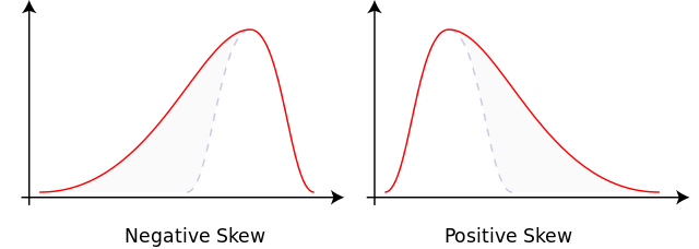
Because it is a probability distribution, the normal curve is a theoretical ideal. It is a type of symmetric distribution that is bell-shaped and has one peak (unimodal) or point of maximum frequency in the middle of the curve. That point is where the mean, median, and mode coincide. If you recall, having the mean, median, and mode at different points reveals a skewed distribution, as shown below in Figures 2 and 3.
Figures 4 and 5 below are sample normal distribution curves. The area under the normal curve contains 100% of all the data. The area is segmented by the Empirical Rule, which states that all observed data for a normal distribution fall within three standard deviations from the mean:
- 68% of the data falls between -1 and +1 standard deviations from the mean.
- 95% of the data falls between -2 and +2 standard deviations from the mean.
- 99.7% percent of the data falls between -3 and +3 standard deviations from the mean.
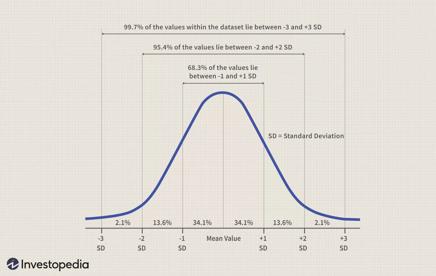
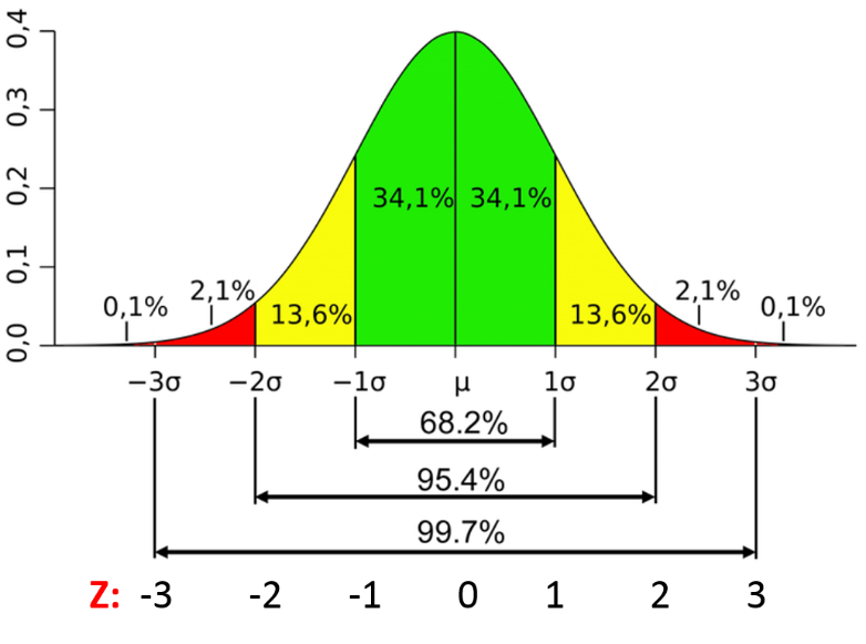
As shown in Figure 5 below, a constant proportion of the total area under the normal curve will lie between the mean and any given distance from the mean as measured in deviation units. Thus, the area under the normal curve between the mean and the point 1 above the mean always turns out to include 34% of the total cases, regardless of the variable of interest. The symmetrical shape of the normal curve means that there is an identical proportion of cases (34%) below the mean. But “What do we do to determine the percent of cases for distances lying between any two score values that do not fit precisely as one, two, three standard deviations from the mean?” To determine, for example, the exact percentage of 1.4 standard deviations from the mean, we would use Percentage Breakdown of Area Under the Normal Curve. Corresponding to the 1.4 standard deviations from the mean includes 41.92% of the total area under the curve.
Now Try It Yourself
3.5 The Standard Normal Distribution
There are infinitely many normal distributions, each with its own mean and standard deviation. The standard normal distribution has a mean of 0 and a standard deviation of 1. We can use the standard score, or z-score, to represent the number of standard deviations a value, x, lies from the mean, µ. To find the z-score for a value, the formula below is used:
[latex]z=\frac{Value-Mean}{Standard\; Deviation}=\frac{x-\mu}{\sigma}[/latex]
A z-score can be positive, negative, or zero. If positive, the corresponding x-value is greater than the mean. When z is negative, the corresponding x-value is less than the mean. If zero, the corresponding x-value is equal to the mean. z-scores can be used as descriptive statistics and as inferential statistics. As descriptive statistics, z-scores describe exactly where each individual is located. As inferential statistics, z-scores determine whether a specific sample is representative of its population or is extreme and unrepresentative.
The Role of Z-Scores in Measuring Malnutrition in Children:
Applying the Equity Lens
The World Health Organization (WHO) defines malnutrition as deficiencies or excesses in nutrient intake, imbalance of essential nutrients, or impaired nutrient utilization. In the area of child health and nutrition, the z-score is the positive or negative standard deviation of a particular child with respect to the median of a carefully selected sample or a predetermined population. WHO categorizes malnutrition in children as severe if the z-score (weight for height and height for age) is less than –3 standard deviations, moderate if the z-score (weight for height and height for age) is between –2 and –3 standard deviations, and mild malnutrition if values are between –2 standard deviations to –1 standard deviation. The criteria for a malnutrition diagnosis are weight loss, low body mass index (BMI), reduced muscle mass, reduced food intake or assimilation, and disease burden/inflammation.
Malnutrition in children is a public health problem in many developing countries such as India. According to Narayan et al. (2019)[3], reports of the National Health & Family Survey, United Nations International Children’s Emergency Fund, and WHO have highlighted that rates of malnutrition among adolescent girls, pregnant and lactating women, and children are alarmingly high in India. Factors responsible for malnutrition in the country include the mother’s nutritional status, lactation behavior, women’s education, and sanitation. These affect children in several ways, including stunting, childhood illness, and retarded growth.
Commentary by the Author: Several years ago, I was invited by The PRASAD Project[4] I worked in India to provide hospital planning-administration consulting support for a new hospital in the Tansa Valley of Maharashtra, India. The Shree Muktananda Mobile Hospital, which began in 1978, is one of PRASAD’s first healthcare initiatives in the Tansa Valley. I rode on the mobile hospital bus every day and saw first-hand how doctors and nurses treated infectious diseases, chronic diseases (such as diabetes and hypertension), skin illnesses, and general health care. Since 1978, over 1,000,000 people have received screenings, medical care, and health education from the Shree Muktananda Mobile Hospital. In addition, PRASAD started its Milk and Nutrition Program for children in 1980. In 1990, volunteers organized the first Eye Camp in India. In 2002, the Maternal and Child Health Program began. In 2004, the HIV Program started, and since then, it has brought the prevalence rate below India’s national level. Before PRASAD began offering programs in the Tansa Valley, most children in the area were malnourished, adults battled untreated tuberculosis and heart disease, and many endured lives of blindness caused by cataracts.
The Anukampaa Health Center is home to PRASAD’s Tuberculosis Program. The disease accounts for more casualties than any other infectious disease in India, claiming a life every minute. Doctors at the Health Center have achieved a tuberculosis cure rate of 95 percent, surpassing the Indian government’s benchmark of 85 percent. In 2010, the World Health Organization and the Indian government’s Revised National TB Control Program recognized the PRASAD program as a Designated Microscopy and Treatment Center.
Now Try It Yourself
| Regions | June | July | August | September |
| Northwest India | 53.1 | 213.8 | 207.2 | 121.0 |
| Central India | 117.4 | 350.8 | 427.7 | 367.3 |
| South Peninsula | 112.3 | 194.3 | 296.1 | 238.2 |
| East & Northeast India | 223.1 | 481.9 | 213.6 | 325.1 |
| Total | 505.9 | 1240.8 | 1144.6 | 1051.6 |

3.6 Blending Probability with Social Justice Issues
A powerful example of social justice is the role of race in the conviction of innocent people. According to Gross et al. (2022)[5], “as of August 8, 2022, the National Registry of Exonerations listed 3,200 defendants who were convicted of crimes in the United States and later exonerated because they were innocent; 53% of them were Black, nearly four times their proportion of the population, which is now about 13.6%.” The National Registry of Exonerations tracks all known wrongful convictions in the United States since 1989.
The Report was made through the joint efforts of the University of California Irvine Newkirk Center for Science and Society, the University of Michigan Law School, and Michigan State University College of Law. The Registry’s first Report on race and wrongful convictions was released in 2017. The September 2022 Report contains more information and detail than the 2017 Report, along with improved data.
When hearing this information, our reaction could be, “Well, given the extent of structural racism in our society and how race is a proxy for criminality in the criminal legal system, this seems quite probable.” We engage in statistical probabilistic thinking unconsciously when we also hear about racial profiling or “driving while Black or Brown”. Black and Hispanic males have complained, filed suit, and organized against what they believe are racist police practices: being stopped, searched, harassed, and sometimes arrested solely because they “fit” a racial profile. So, when we hear on the news about another killing of a young black male by a police officer or a neighbor, we are not surprised because such events have become normalized or “highly likely” in the United States.
Putting emotions aside, there are concepts in statistics that we can apply as we blend probabilistic thinking with social justice issues. They are randomness, experimental and theoretical probability, simulation, sample size, and the law of large numbers. Let’s take, for example, the principle of randomness, which is the heart of statistics that underpins much of our knowledge. It is the apparent or actual lack of pattern or predictability of information or event. Randomness in probability describes a phenomenon in which the outcome is uncertain, but there is a regular distribution of relative frequencies in a large number of repetitions. In the instance of racial profiling, such occurrences do not seem to be random but have more of a definite plan, purpose, or pattern. We have seen in the multitude of racial profiling cases that there is both a predictable short- and long-term pattern that can be described by the distribution of outcomes, namely, being stopped, searched, harassed, and sometimes arrested solely because Black and Brown males “fit” a racial profile.
Chapter 3: Summary
In this chapter, we learned that probability is a statistical term used to express the likelihood that an event will happen. The probability of an event can be calculated by the probability formula by simply dividing the favorable number of outcomes by the total number of possible outcomes. The closer the probability is to zero, the less likely it is to happen, and the closer the probability is to one, the more likely it is to happen. The total of all the probabilities for an event is equal to one.
We also learned that the normal curve is a probability distribution in which the total area under the curve equals 100%. It contains a central area surrounding the mean, where scores or observations occur most frequently, and smaller areas toward either end, where there is a gradual flattening out and, thus, a smaller proportion of extremely high and low scores. From a probability perspective, we have seen in previous graphs that probability decreases as we travel away from the mean in either direction. Thus, 68% of the cases falling within -1 and +1 standard deviations is like saying that the probability is approximately 68 in 100 that any given raw score will fall within this interval.
In Chapter 4, we will move from descriptive statistics, where we acquired tools to describe a data set, to inferential statistics, where we make inferences based on a data set. The goal is to discover a general pattern about a large group while studying a smaller group of people in the hope that results can be generalized to the larger group. The most common methodologies in inferential statistics are hypothesis testing, confidence intervals, and regression analyses, which will be covered in subsequent chapters.
Remember: It is not solely about the destination. It is also about the journey of gaining a critical statistical perspective that incorporates and facilitates awareness of social justice issues. I hope you are enjoying your journey and seeing how statistics is a tool to help affect social change in society.
- Benecchi L (2021). Recidivism Imprisons American Progress. Harvard Political Review. https://harvardpolitics.com/recidivism-american-progress/ Retrieved on June 8, 2023. ↵
- Levin J & Fox JA (2006). Elementary Statistics in Social Research. Pearson, Inc., Boston, MA; Tenth Edition. ↵
- Narayan J, John D & Ramadas N (2019). Malnutrition in India: Status and Government Initiatives. Journal of Public Health Policy, 40, pages126–141. ↵
- . PRASAD is a philanthropic expression of the Siddha Yoga mission. Gurumayi Chidvilasananda, the spiritual head of the Siddha Yoga path, started the PRASAD Project in 1992. I had the honor and privilege to serve Gurumayi on this project, which has had the most amazing impact on my life—both personally and professionally. PRASAD is a leading humanitarian organization that effectively addresses health inequalities and the social determinants of health among the poorest of the poor in India. My experience with PRASAD is the genesis and motivation for this book. ↵
- Gross SR, Possley M, Otterbourg K, Stephens K, Paredes JW & O’Brien B (2022). Race and Wrongful Convictions in the United States 2022. National Registry of Exonerations, September. ↵
