
5 Significance of Statistical Inference Methods
This chapter is a continuation of the previous chapter on inferential statistics.
Learning Outcomes
- Significance of Statistical Inference Methods
- Confidence Intervals
- Hypothesis Testing
- Type I and Type II Errors
- Scientific Racism
The importance of statistical inference is grounded in several assumptions. First, it addresses a particular type of uncertainty, namely that caused by having data from random samples rather than having complete knowledge of entire populations, processes, or distributions. Second, we cannot build statistical inference without first building an appreciation of sample versus population, of description versus inference, and of characteristics of samples giving estimates of characteristics of populations. Third, any conceptual approach to statistical inference must flow from some essential understanding of the nature and behavior of sampling variation. Finally, statistical inference is viewed as both an outcome and a reasoned process of creating or testing probabilistic generalizations from data. The prior four chapters introduced you in varying degrees to these points.
In this chapter, you will see how sampling distributions are used to test hypotheses and construct confidence intervals. Topics discussed in this chapter are:
- Implicit Assumptions in Making Statistical Inferences
- Significance of Statistical Inference Methods
- Confidence Intervals
- Tests of Significance
5.1. Implicit Assumptions in Making Statistical Inferences
One of the statistician’s most important roles is the upfront contribution of planning a study, which includes identifying the implicit assumptions when making statistical inferences. It is important that these assumptions are met, and if they are not, the statistical inferences can result in seriously flawed conclusions in the study. According to Hahn & Meeker (1993)[1], the first assumption is that the target population has been explicitly and precisely defined. The second assumption is that a specific listing (or another enumeration) of the population from which the samples have been selected has been made. Third, the data are assumed to be a random sample of the population. The assumption of random sampling is critical. When the assumption of random sampling (or randomization) is not met, inferences to the population become difficult. In this case, statisticians should describe the sample and population in sufficient detail to justify that the sample was at least representative of the intended population.
5.2. The Significance of Statistical Inference Methods
You have now acquired a clear understanding of the difference between a sample (the observed) and the population (the unobserved). The extent to which credence should be placed in a given sample statistic as a description of the population parameter is the problem of inferring from the part to the whole. This is sometimes called the problem of inductive inference, or the problem of generalization.
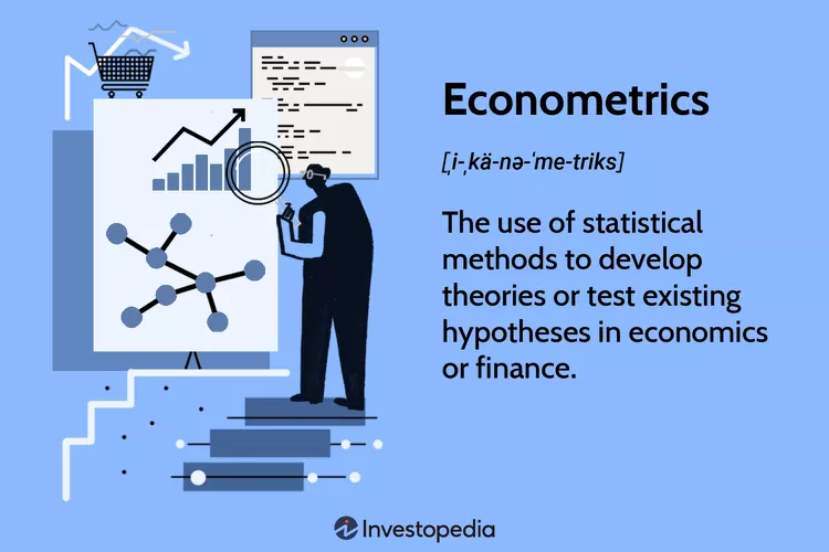
Using the field of Econometrics[2] as an example, Keuzenkamp & Magnus (1995)[3] describes the four types of statistical testing:
- Theory Testing: This method consists of formulating hypotheses from which predictions of novel facts are deduced (the consequences).
- Validity Testing: Performed in order to find out whether the statistical assumptions underlying some models are credible. In order to pursue a theory test, one first must be sure of the validity of the statistical assumptions that are made.
- Simplification Testing: Simplicity matters. Simple models are typically preferred to complex ones. Rather than testing from general to simple, statisticians perform iterative simplification searches. In the study of statistics, we focus on mathematical distributions for the sake of simplicity and relevance to the real world. Understanding these distributions enables us to visualize the data more easily and build models more quickly.
- Decision-Making: Based on statistical acceptance rules, this method can be important for process quality control and can be extended to appraising theories.
The type of statistical test one uses depends on the type of study design, number of groups of comparison, and type of data (i.e., continuous, dichotomous, and categorical) (Parab & Bhalerao 2010).[4]
Subsequent sections will discuss statistical inference methods that use the language of probability to estimate the value of a population parameter. The two most common methods are confidence intervals and tests of significance.
5.2(a). Confidence Intervals (CI)
A confidence interval (CI), in statistics, refers to the probability that a population parameter falls between two set values. The sample is used to estimate the interval of probable values of the parameters of the population. It is a matter of convention to use the standard 95% confidence interval having the probability that there are 95 chances out of 100 of being right. There are five chances out of 100 of being wrong. Even when using the 95%[5] confidence interval, we must remember that the sample mean could be one of those five sample means that fall outside the established interval. A statistician never knows for sure.
According to Zhang, Hanik & Chaney (2008)[6], the CI has four noteworthy characteristics:
- For a given sample size, at a given level of confidence, and using probability sampling, there can be infinitely many CIs for a particular population parameter. The point estimates and endpoints of these CIs vary due to sampling errors that occur each time a different sample is drawn.
- The CI reported in a certain research study is just one of these infinitely many CIs.
- The percentage of these CIs that contain the population parameter is the same as the level of confidence.
- Whether a certain CI reported by a research study contains the population parameter is unknown. In other words, the level of confidence is applied to the infinitely many CIs, rather than a single CI reported by a single study.
A Confidence Interval to Estimate Population Poverty in the United States:
Applying the Equity Lens
The U.S. Census Bureau routinely uses confidence levels of 90% in their surveys. “The number of people in poverty in the United States is 35,534,124 to 37,315,094″ means (35,534,124 to 37,315,094) is the confidence interval. Assuming the Census Bureau repeats the survey 1,000 times, the confidence level of 90% means that the stated number is between (35,534,124 to 37,315,094) at least 900 times. Maybe 36,000,000 people are in poverty–maybe less or greater. Any number in the interval is as expected.
Any confidence interval has two parts: an interval calculated from the data and a confidence level C. The confidence interval often has the form:
estimate [latex]\pm[/latex] margin of error
The confidence level is the success rate of the method that produces the interval, that is, the probability that the method will give a correct answer. The statistician chooses the confidence level, and the margin of error follows from this choice. When the data and the sample size remain the same, higher confidence results in a larger margin of error. There is a tradeoff between the confidence level and the margin of error. To obtain a smaller margin of error, the statistician must be able to accept a lower confidence. As the sample size increases, the margin of error gets smaller.
A level C confidence interval for the mean µ of a Normal population with known standard deviation σ, based on a simple random sample of size n, is given by:
[latex]\bar{X}\pm z*\frac{\sigma}{\sqrt{n}}[/latex]
The critical value z* is chosen so that the standard Normal curve has an area C between – z* and z*. Below are the entries for the most common confidence levels:
| Confidence Level C | 90% | 95% | 99% |
|---|---|---|---|
| Critical value z* | 1.645 | 1.960 | 2.576 |
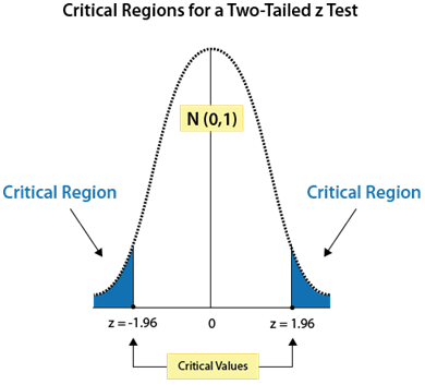
We know from the Central Limit Theorem (chapter 4) that when n ≥ 30, the sampling distribution of sample means approximates a normal distribution. The level of confidence C is the area under the standard normal curve between the critical values, -zc and zc. Critical values are values that separate sample statistics that are probable from sample statistics that are improbable, or unusual. For instance, if C =95%, then 2.5% of the area lies to the left of -zc = -1.960 and 2.5% lies to the right of zc = 1.960, as shown in the Table below:
If C = 95%, then:
[latex]1-C=.05[/latex]
[latex]\frac{1}{2}(1-C)=.025[/latex] [Area in one tail]
[latex]-z_{c}=-1.960[/latex] [Critical value separating left tail in the normative curve]
[latex]z_{c}=1.960[/latex] [Critical value separating righttail in the normative curve]
An example of the meaning of the 95% confidence interval is as follows:
Suppose a medical researcher is interested in the prenatal care received by pregnant women in the inner city of Philadelphia. She breaks down the various sections of North Philly and computes the average number of gynecological check ups per pregnancy for all possible samples of size 20 and constructs the 95% confidence intervals using these sample means. Then 95% of these intervals would contain µ [population parameter]and 5% would not. Note that we cannot say that the probability is .95 that the interval from 2.6 to 3.4 gynecological checkups, for example, contains µ. Either the interval contains µ or it does not.
The 95% confidence interval of 2.6 to 3.4 was calculated based on the average number of gynecological check ups per pregnancy being 3, with a standard deviation of 1.
[latex]\bar{X}\pm z*\frac{\sigma }{n}[/latex]
[latex]=3\pm 1.96\frac{1}{\sqrt{20}}[/latex]
[latex]=2.6[/latex] to [latex]3.4[/latex]
An Equitable Transition to Electric Transportation:
Applying the Equity Lens
The newness of electric vehicles, their high upfront cost, the need for charging access, and other issues mean that equity has been overlooked (Hardman, Fleming, Khare & Ramadan 2021)[7]. Electric vehicle buyers are mostly male, high-income, highly educated homeowners who have multiple vehicles in their household and have access to charging at home. There is a need for a more equitable electric vehicle market so that the benefits of electrification are experienced by all and so that low-income households are not imposed with higher transportation costs. Low-income households, including those in underrepresented communities and in disadvantaged communities, could benefit from transportation electrification. These households are impacted by transportation emissions as they are more likely to reside in or near areas of high traffic and spend a higher proportion of their household income on transportation costs. Households in these communities are less likely to have charging at home or be able to afford to install home charging, have smaller budgets for vehicle purchases, and have fewer vehicles in their household. They are also less likely to have a regular place of work, which means they may not have workplace charging access (an alternative to home charging). These factors make plug-in electric vehicle (PEV) ownership more challenging,
A Step-by-Step Illustration: 95% Confidence Interval Using z
Suppose that the automobile company, Honda, wishes to address the mobility needs of underserved communities. As a separate research project, the company will work on the barriers and enablers of electrification. Until then, Honda determines the expected miles per gallon for a new 2025 HRV model that is designed to be far more affordable and efficient for low-income buyers. The company statistician knows from years of experience that not all cars are equivalents. She believes that a standard deviation of 4 miles per gallon (σ = 4) is expected due to parts and technician variations. To estimate the mean miles per gallon for the new model, she test runs a random sample of 100 cars off the assembly line and obtains a sample mean of 26 miles per gallon.
The following are steps to obtaining a 95% confidence interval for the mean miles per gallon for all cars of the HRV model.
Step 1: Obtain the mean for a random sample (which has already been provided).
[latex]N=100;\bar{X}=26[/latex]
Step 2: Calculate the standard error of the mean, knowing that σ = 4.
[latex]\sigma _{\bar{X}}=\frac{\sigma }{\sqrt{n}}[/latex]
[latex]=\frac{4}{\sqrt{100}}[/latex]
[latex]=\frac{4}{\sqrt{10}}[/latex]
[latex]=.4[/latex]
Step 3: Calculate the margin of error by multiplying the standard error of the mean by 1.96, the value of z for a 95% confidence interval.
Margin of error [latex]=1.96\sigma _{\bar{X}}[/latex]
[latex]=1.96(.4)[/latex]
[latex]=.78[/latex]
Step 4: Add and subtract the margin of error from the sample mean to find the range of mean scores within which the population mean is expected to fall with 95% confidence.
95% Confidence Interval [latex]=\bar{X}\pm 1.96\sigma _{\bar{X}}[/latex]
[latex]=26\pm .78[/latex]
[latex]=25.22[/latex] to [latex]26.78[/latex]
Thus, the statistician can be 95% confident that the true mean miles per gallon for the new 2025 HRV model (µ) is between 25.22 and 26.78.
Important! After constructing a confidence interval, the results must be interpreted correctly. Consider the 95% confidence interval constructed in the above example. Because µ is a fixed value predetermined by the population, it is in the interval or not. It is not correct to say, “There is a 95% probability that the actual mean will be in the interval (25.22, 26.78).” This statement is wrong because it suggests that the value µ can vary, which is not true. The correct way to interpret this confidence interval is to say, “With 95% confidence, the mean is in the interval (25.22, 26.78).” This means that when a large number of samples are collected and a confidence interval is created for each sample, approximately 95% of these intervals will contain µ.
Now Try It Yourself
5.2(b). Tests of Significance
The second type of statistical inference is tests of significance. The tests of significance aid the statistician in making inferences from the observed sample to the unobserved population.
The test of significance provides a relevant and useful way of assessing the relative likelihood that a real difference exists and is worthy of interpretive attention, as opposed to the hypothesis that the set of data could be an arrangement lacking any type of pattern. The basic idea of statistical tests is like that of confidence intervals: what would happen if we repeated the sample many times?
A statistical test starts with a careful statement of the claims a statistician wants to compare. Because the reasoning of tests looks for evidence against a claim, we start with the claim we seek evidence against, such as “no effect or “no difference.”
5.2(b)(1). The Null Hypothesis: No Difference Between Means
A statistical hypothesis test is a method of statistical inference used to decide whether the data at hand sufficiently supports a particular hypothesis.[8] In terms of selecting a statistical test, the most important question is, “What is the main hypothesis for the study?” In some cases, there is no hypothesis; the statistician just wants to “see what is there.”
On the other hand, if a scientific question is to be examined by comparing two or more groups, one can perform a statistical test. For this, initially, a null hypothesis needs to be formulated, which states that there is no difference between the two groups. It is expected that at the end of the study, the null hypothesis is either rejected or not rejected (Parab & Bhalerao 2010).
The claim tested by a statistical test is called the null hypothesis. The test is designed to assess the strength of the evidence against the null hypothesis. The claim about the population that we are trying to find evidence for is the alternative hypothesis. The alternative hypothesis is one-sided if it states that the parameter is larger than or smaller than the null hypothesis value. It is two-sided if it states that the parameter is different (larger or smaller) from the null value (Moore, Notz & Fligner 2013).
The null hypothesis is abbreviated as Ho, and the alternative hypothesis as Ha. Ho is a statistical hypothesis that contains a statement of equality, such as ≤, =, or ≥. Ha is the complement of the null hypothesis. It is a statement that must be true if Ho is false. It contains a statement of strict inequality, such as >, ≠, or <. Ho is read as “H naught.” Ha is read as “H sub-a.”
You always begin a hypothesis test by assuming that the equality condition in the null hypothesis is true. When you perform a hypothesis test, you make one of two decisions:
- Reject the null hypothesis or
- Fail to reject the null hypothesis.
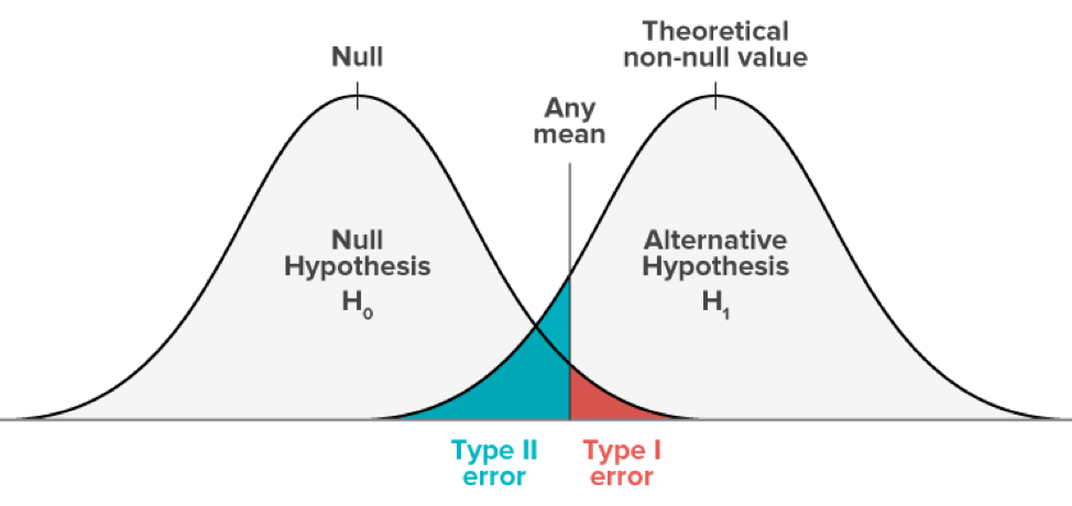
Know that because a decision is based on a sample rather than the entire population, there is the possibility of making the wrong decision. The only way to be absolutely certain of whether Ho is true or false is to test the entire population, which, in reality, may not be feasible. So, the statistician must accept the fact that the decision might be incorrect. As shown in Figure 2 below, there are two types of errors that can be made:
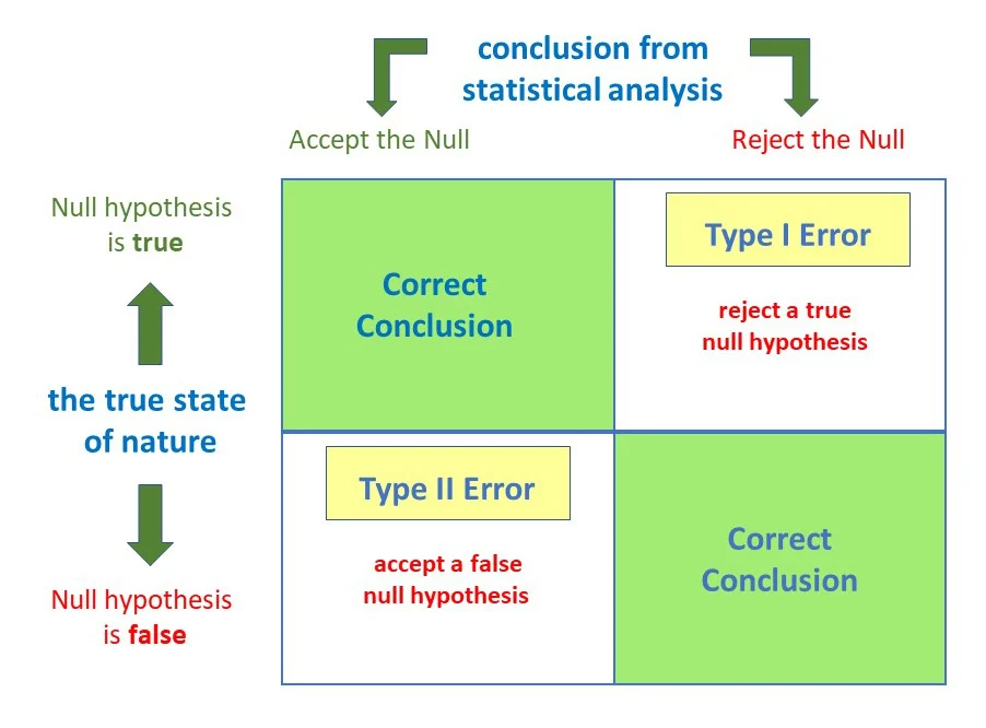
A Type I Error occurs if the null hypothesis is rejected when it is true.
A Type II Error occurs if the null hypothesis is not rejected when it is false.
In a hypothesis test, the level of significance is the maximum allowable probability of making a Type I error. It is denoted by α, the lowercase Greek letter alpha. The probability of a Type II error is denoted by β, the lowercase Greek letter beta. By setting the level of significance at a small value, the probability of rejecting a true null hypothesis will be small. The commonly used levels of significance are: α = 0.01; α = 0.05; and α = 0.10. When α is decreasing (the maximum probability of making a Type I Error), it is likely that β is increasing. The value 1 – β is called the power of the test. It represents the probability of rejecting the null hypothesis when it is false.
Hypotheses always refer to the population, not to a particular outcome. They are stated in terms of population parameters. Thus, for no difference between means, the null hypothesis can be symbolized as
µ1 = µ2
where µ1 = mean of the first population
µ2 = mean of the second population
Now Try It Yourself[9]
A test is based on a test statistic that measures how far the sample outcome is from the value stated by Ho. The P-value of a test is the probability that the test statistic will take a value at least as extreme as that actually observed. Small P-values indicate strong evidence to reject the null hypothesis provided by the data. However, a very low P-value does not constitute proof that the null hypothesis is false, only that it is probably false. Large P-values fail to give evidence against Ho. The most important task is to understand what a P-value says.
If the P-value is as small or smaller than a specified value α (alpha), the data are statistically significant at significance level α.
Decision Rule Based on P-Value[10]
To use a P-value to decide in a hypothesis test, compare the P-value with α.
If P ≤ α, then reject Ho.
If P > α, then fail to reject Ho.
When to Use the P-Value and How to Interpret It[11]
“Assume there is data collected from two samples and that the means of the two samples are different. In this case, there are two possibilities: the samples really have different means (averages), or the other possibility is that the difference that is observed is a coincidence of random sampling. However, there is no way to confirm any of these possibilities.
All the statistician can do is calculate the probabilities (known as the “P” value in statistics) of observing a difference between sample means in an experiment of the studied sample size. The value of P ranges from zero to one. If the P value is small, then the difference is quite unlikely to be caused by random sampling, or in other words, the difference between the two samples is real. One has to decide this value in advance, i.e., at which smallest accepted value of P, the difference will be considered as a real difference.
The P value represents a decreasing index of the reliability of a result. The higher the P value, the less we can believe that the observed relation between variables in the sample is a reliable indicator of the relation between the respective variables in the population. Specifically, the P value represents the probability of error that is involved in accepting our observed result as valid, i.e., as “representative of the population.” For example, a P value of 0.05 (i.e., 1/20) indicates that there is a 5% probability that the relation between the variables found in our sample is a “fluke.” In other words, assuming that in the population, there was no relation between those variables whatsoever, and we were repeating experiments such as ours one after another, we could expect that approximately in every 20 replications of the experiment, there would be one in which the relation between the variables in question would be equal to or stronger than in ours. In many areas of research, the P value of 0.05 is customarily treated as a “cut-off” error level.”
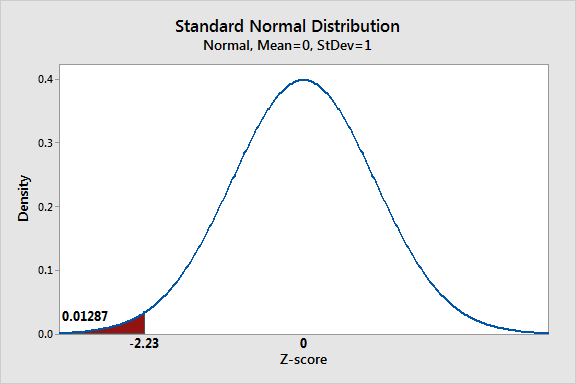
The P-value of a test depends on the nature of the test. As shown in Figure 3 below, there are three types of hypothesis tests—left-tailed, right-tailed, and two-tailed (where evidence that would support the alternative hypothesis could lie in either tail of the sampling distribution).
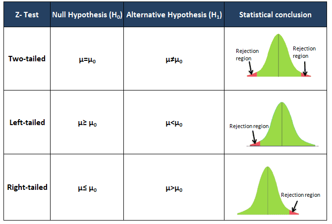
In a left-tailed test, the alternative hypothesis Ha contains the less-than inequality symbol (<):
Ho: µ ≥ k
Ha: µ < k
In a right-tailed test, the alternative hypothesis Ha contains the greater-than-inequality symbol (>):
Ho: µ ≤ k
Ha: µ > k
In a two-tailed test, the alternative hypothesis Ha contains the not-equal-to symbol (≠):
Ho: µ = k
Ha: µ ≠ k
Steps in Hypothesis Testing
- State mathematically and verbally the null and alternative hypotheses.
Ho : ? Ha : ?
- Specify the level of significance.
α = ?
- Obtain a random sample from the population.
- Calculate the sample statistic (such as x̅, p̂, s2) corresponding to the parameter in the null hypothesis (such as µ, p, or σ2). This sample statistic is called the test statistic.
- With the assumption that the null hypothesis is true, the test statistic is then converted to a standardized test statistic, such as z, t (student’s t-test) or χ2 (chi-square). The standardized test statistic is used in making the decision about the null hypothesis.
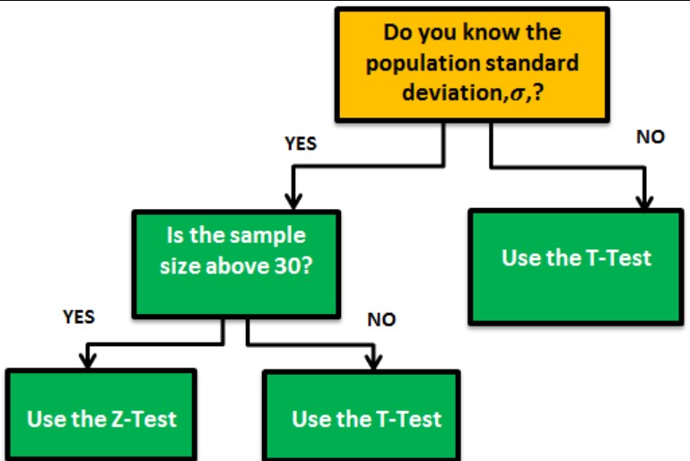
Student’s t Test[12]: A t-test may be used to evaluate whether a single group differs from a known value (a one-sample t-test), whether two groups differ from each other (an independent two-sample t-test), or whether there is a significant difference in paired measurements (a paired, or dependent samples t-test). t-tests rely on an assumed “null hypothesis.” You have to decide whether this is a one-tail (Is it greater or less than?) or a two-tail test (Is there a difference?) and choose the level of significance (Greek letter alpha, α). An alpha of .05 results in 95% confidence intervals and determines the cutoff for when P-values are considered statistically significant.
The assumptions of a t-test are:
- One variable of interest.
- Numeric data.
- Two groups or less.
- Random sample.
- Normally distributed.
Chi-Square Test (χ2): a statistical test commonly used to determine if there is a significant association between two variables.
For example[13], many Black and Latinx organizations receive relatively small program grants. To reverse this trend and to engender sustainability, foundations could create grantee cohorts in traditionally underserved communities and neighborhoods. This neighborhood cohort approach has been used successfully by foundations for decades for a variety of reasons, such as achieving efficiency and promoting collaboration. Unbound Philanthropy’s Good Neighbor Committee, a staff initiative dedicated to grantmaking in the New York City metro, sought to reduce gang violence in central Long Island by supporting several organizations that were working on the problem from different angles. These included a youth development organization and a parent advocacy organization. The Chi-Square Test for Independence tests two hypotheses:
Null Hypothesis: There is not a significant association between variables, the variables are independent of each other. Any association between variables is likely due to chance and sampling error. For example, there is no significant association between Organization A (a youth development organization) and Organization B (a parent advocacy organization). Each organization’s ability to reduce gang violence has nothing to do with the other.
Alternative Hypothesis: There is a significant association (positive or negative) between variables, the variables are independent of each other. Any association between variables is not likely due to chance and sampling error. For example, there is a significant association between Organization A (a youth development organization) and Organization B (a parent advocacy organization). Each organization’s ability to reduce gang violence, to some degree, impacts the other.
- Find the P-value.
- Use this decision rule: If P-value is less than or equal to the level of significance, then reject the null hypothesis. If P-value is greater than the level of significance, then fail to reject the null hypothesis.
- Write a statement to interpret the decision in the context of the original claim.
Now Try It Yourself
The Financial Risk Tolerance of Blacks, Hispanics, and Whites:
Applying the Equity Lens
Yao, Gutter & Hannah (2005)[14] studied the effects of race and ethnicity on financial risk tolerance. Risk attitudes may affect investment behavior, so having an appropriate willingness to take financial risk is important in achieving investment goals. In turn, investment choices can affect retirement well-being, and, more specifically, the retirement adequacy of different racial and ethnic groups. This study focused on the expressed risk tolerance of Hispanics and Blacks compared to Whites because of the implications of investment behavior for future wealth differences and improving financial education programs.
Descriptive Statistics Results : White respondents are significantly more likely to be willing to take some risk (59%) than are Blacks (43%), who are significantly more likely to be willing to take some risk than Hispanics (36%). However, the pattern is reversed for willingness to take substantial risk, with only 4% of Whites but 5% of Blacks and 6% of Hispanics willing to take substantial risk.
Hypotheses Testing Results: The hypotheses are confirmed for substantial risk. Table 2 below summarizes the hypothesis tests. Based on the z-tests, Whites are significantly more likely than Blacks, and Blacks are significantly more likely than Hispanics to be willing to take some financial risks. For substantial risk, the results are the opposite of the hypotheses, as Whites are significantly less likely than Blacks and Hispanics to be willing to take substantial financial risks; and the difference between Hispanics and Blacks is not significant. For high risk, the hypothesis that Whites are more likely to be willing to take risks than the other two groups are confirmed, but Hispanics are as willing to take high risks as Blacks.
| Financial Risk tolerance levels | Z-test results | Logit results |
|---|---|---|
| Substantial | Not accepted: Hispanics = Blacks > Whites | Not accepted: Hispanics = Blacks > Whites |
| High | Partially Accepted: Whites > Hispanics = Blacks | Not accepted: Hispanics = Blacks = Whites |
| Some | Accepted: Whites > Blacks > Hispanics | Accepted: Whites > Blacks > Hispanics |
> : Significantly greater at the .05 level or better
= : Not significantly different at the .05 level
Below are a sample of hypotheses found in the research literature on race and ethnicity and their intersection with other variables, such as age, socioeconomic status, and sexual preference:
- Contact Hypothesis: Interracial contact is associated with more positive racial attitudes, especially among Whites and some effects are appreciable.
- Cumulative Disadvantage Hypothesis: Predicts that initial advantages and disadvantages compound and produce diverging health trajectories as individuals age. Rationale: Given the structural disadvantages that people of color face across multiple domains of the life course, the cumulative disadvantage hypothesis predicts that racial-ethnic health disparities increase with age. (Brown, O’Rand & Adkins (2012)[15].
- Ethnicity Hypothesis: Ethnic minorities engage more in social activities than Whites of comparable socioeconomic status. Rationale: The relatively smaller, more cohesive ethnic group is able to exert pressure on the individual member to conform to the norms of the respective ethnic affiliation. (Antunes and Gaitz 1975)[16].
- LGBT-POC (People of Color) Hypothesis: These individuals may experience unique stressors associated with their dual minority status, including simultaneously being subjected to multiple forms of microaggressions (brief, daily assaults which can be social or environmental, verbal or nonverbal, intentional or unintentional). Within LGBT communities, LGBT-POC may experience racism in dating relationships and social networks. Rationale: Racial/ethnic minority individuals have reported exclusion from LGBT community events and spaces. For example, certain gay bars have been noted for refusing entry of African Americans and providing poorer service to Black patrons. (Balsam et al. 2011)[17].
- Persistent Inequality Hypothesis: Predicts that racial-ethnic inequalities in health remain stable with age. Rationale: Socio-economic conditions and race-ethnicity are considered “fundamental causes” of disease and illness because of their persistent association with health over time regardless of changing intermediate mechanisms. (Brown, O’Rand & Atkins (2012).
- Statistical Discrimination or Profiling Hypothesis: In this situation, an individual or firm uses overall beliefs about a group to make decisions about an individual from that group. The perceived group characteristics are assumed to apply to the individual. Thus, statistical discrimination may result in an individual member of the disadvantaged group being treated in a way that does not focus on his or her own capabilities. (National Academies Press 2004)[18].
- Weathering Hypothesis: Chronic exposure to social and economic disadvantage leads to accelerated decline in physical health outcomes and could partially explain racial disparities in a wide array of health conditions. (Forde, Crookes, Suglia & Demmer 2019)[19].
Chapter 5: Summary
Rather than summarize the content of this chapter, I decided to do something different. I would like to share with you something that I came across while researching articles for this book. I was introduced to the term scientific racism by Jay (2022)[20], which was deeply concerning. Its genesis is described in the following:
“Scientific racism,” or more accurately pseudo-scientific racism (because racism is not scientific), was a way in which European colonial governments — and the statisticians they hired to do government surveys and data collection — justified their racist policies by using statistical measurements, often in an extremely biased and incorrect way. For example — if you’ve ever heard of the infamous “skull measurements” used by European pseudo-scientists in the colonial era to try to demonstrate a (fake) correlation between skull size and intelligence — you should know they did that in order to put scientific backing behind claims such as “Africans, Native Americans, and Asians are less intelligent than Europeans due to smaller size.” Of course, these claims are completely unscientific and baseless — but using scientific terminology and measurements as a backing was a way to soothe their guilty conscience.
…But how does this tie in with racism? Well — when colonial European “scientists” began measuring the heights, weights, and appearances of “races” in the world, they leaned on European statisticians like Galton to make conclusions based on the data. He and his contemporaries believed that the measurements of people in each of their “races” would follow a bell curve — the normal distribution.
If these “racial measurements” followed a normal distribution — well, since every normal curve has a specific mean and standard deviation — it “follows” that each “race” of people has an “average look.” If this logic already sounds creepy to you — that’s because it IS — and it’s frankly mind-blowing how some of these statisticians convinced themselves their research was wholly “scientific.”
Author’s Comment: The above reminds us that the journey of “equity-mindedness” is really about doing anti-racism, anti-oppression, and anti-colonialism work. Thus, statistics must be socially just in its methods as well as its intentions.
Writing this OER book has reinforced the importance of upholding dharma (ethical and moral righteousness) when planning and implementing a study. Not only do we have to be careful about “bias creep,” but be careful about the unintended deleterious effects of conclusions reached.
Thank you all for staying committed to this journey! I take this opportunity to acknowledge the group Sweet Honey in the Rock, which celebrates its 50th Anniversary this year of singing social justice songs. Their debut began in 1973 at a workshop at Howard University, a historically Black college in Washington, DC. It was their creative songs that motivated me each day to write this OER book.

- Hahn GJ & Meeker WQ (1993). Assumptions for Statistical Inference. The American Statistician, February, Vol. 47, No.1. ↵
- , the Author’s undergraduate degree is in Economics and Psychology. In graduate school, served as a Teaching Assistant in the graduate-level course on Econometrics. ↵
- Keuzenkamp HA & Magnus JR (1995). On Tests and Significance in Econometrics. Journal of Econometrics, 67, 5-24. ↵
- Parab S & Bhalerao S (2010). Choosing Statistical Tests. International Journal of Ayurveda Research. July-September; 1(3): 187-191. ↵
- , statisticians also use 90% and 99% levels of confidence. ↵
- Zhang J, Hanik BW & Chaney BH (2008). ↵
- Hardman S, Fleming KL, Khare E & Ramadan MM (2021). A Perspective on Equity in the Transition to Electric Vehicles. MIT Science Policy Review, August 30, 2021, Volume 2, 41-52. ↵
- Wikipedia. Statistical Hypothesis Testing. https://en.wikipedia.org/wiki/Statistical_hypothesis_testing. Retrieved on July 4, 2023. ↵
- Problems taken from Levin J & Fox JA (2006). ↵
- Larson R & Farber B (2019). ↵
- Example provided by Parab & Bhalerao (2010). ↵
- GraphPad. The Ultimate Guide to T Tests. https://www.graphpad.com/guides/the-ultimate-guide-to-t-tests#V2hhdCBhcmUgdGhlIGFzc3VtcHRpb25zIGZvciB0IHRlc3RzPw. Retrieved on July 4, 2023. ↵
- Pearce M & Eaton S. Equity, Inclusion and Diversity in Art and Culture Philanthropy. Social Justice Funders Opportunity Brief, No. 3. Brandeis University (Waltham, MA), the Sillerman Center for the Advancement of Philanthropy. https://heller.brandeis.edu/sillerman/pdfs/opportunity-briefs/arts-and-culture-philanthropy.pdf. Retrieved on July 4, 2023. ↵
- Yao R, Gunner MS, & Hanna SD (2005). The Financial Risk Tolerance of Blacks, Hispanics, and Whites. Financial Counseling and Planning, Volume 16 (1), 51-62. ↵
- Brown TH, O’Rand AM & Adkins DE (2012). Race-Ethnicity and Health Trajectories: Tests of Three Hypotheses Across Multiple Groups and Outcomes. Journal of Health and Social Behavior, Volume 53, Issue 3. ↵
- Antunes G & Gaitz C (1975). Ethnicity and Participation: A Study of Mexican Americans, Blacks and Whites. American Journal of Sociology, 80 (March): 1192-1211. ↵
- Balsam KF, Molina Y, Beadnell B, Simoni J & Walters K (2011). Measuring Multiple Minority Stress: The LGBT People of Color Microaggressions Scale. Cultural Diversity Ethnic Minority Psychology, April; 17(2): 163-174. ↵
- National Academies Press (2004). Chapter 4: Theories of Discrimination. In the book, Measuring Discrimination. https://nap.nationalacademies.org/read/10887/chapter/7. Retrieved on July 3, 2023. ↵
- Forde AT, Crookes DM, Suglia SF, & Demmer RT (2019). The Weathering Hypothesis as an Explanation for Racial Disparities in Health. Annals of Epidemiology, May, 33:1. ↵
- Jay R (2022). P-values: A Legacy of “Scientific Racism.” https://towardsdatascience.com/p-values-a-legacy-of-scientific-racism-d906f6349fc7. Retrieved on July 3, 2023. ↵
