
Multiple crossovers: the three-point testcross
The recombination frequency underestimates long map distances as discussed in the previous section. In addition, if multiple crossover events occur between two genes, those crossover events will not be detected using a two-point test cross. This is illustrated in Morgan’s 1923 text, reprinted in Figure 7b from earlier in this chapter. Although two crossovers have occurred between genes W and Br, they would not be counted in a two-point test cross between W and Br because the parental alleles would still appear to be linked. Multiple crossover events are increasingly likely to happen the further apart the genes.
To partially solve this, a three-point test cross can be used. Having a third point intermediate to the other two allows detection of double-crossover events, since the middle gene would be swapped out in the case of a double recombinant. This is also called a trihybrid testcross – you might recall that a trihybrid would be heterozygous for three genes, for example AaBbCc.
An example of a hypothetical three point testcross is shown in Figure 14, reprinted from Online Open Genetics (Nickle and Barrette-Ng)[1]. Here, three traits are tracked in mice: tail length (Long or short), fur color (Brown or white), and whisker length (Long or short).
While a dihybrid testcross gives 4 potential classes of offspring (AB, Ab, aB, ab), a trihybrid testcross potentially gives 8 classes of offspring (ABC, abc, Abc, aBC, aBc, AbC, ABc, abC). The 8 possible classes are shown for the F2 generation in Figure 14.
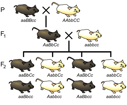
Table 5 gives sample data for the testcross in Figure 14. The parental phenotypes are highlighted. For any testcross with linkage, the parental phenotypes will be the most numerous class.
| Class number | tail phenotype (A) | fur phenotype
(B) |
whisker phenotype
(C) |
gamete from trihybrid | genotype of F2 from test cross | number of progeny |
|---|---|---|---|---|---|---|
| 1 | short | Brown | Long | aBC | aaBbCc | 5 |
| 2 | Long | white | Long | AbC | AabbCc | 38 |
| 3 | short | white | Long | abC | aabbCc | 1 |
| 4 | Long | Brown | Long | ABC | AaBbCc | 16 |
| 5 | short | Brown | short | aBc | aaBbcc | 42 |
| 6 | Long | white | short | Abc | Aabbcc | 5 |
| 7 | short | white | short | abc | aabbcc | 12 |
| 8 | Long | Brown | short | ABc | AaBbcc | 1 |
| Total | No Data | No Data | No Data | No Data |
No Data |
120 |
The rest of the data are analyzed by looking at two genes at a time to calculate recombination frequency. So, for example, we can look at just tail and fur phenotypes, as if we’d never tracked whisker phenotype at all.
The parents for this cross had short tail, Brown fur and Long tail, white fur. Those are highlighted in yellow in Table 6. That means the recombinants are short, white and Long, brown. Those are highlighted in green. There are 30 total recombinant offspring out of 120, or 25%. This means the tail gene (A) and fur gene (B) are 25 map units apart.
We can then repeat this for the remaining pair-wise combinations. Table 7 shows the count for recombination between fur (B) and whisker (C). Table 8 shows the count for recombination between whisker (C) and tail (A).
| Tail (A) | Fur (B) | whisker (C) | # of progeny | Recombinant for tail and fur? | Recombinant for fur and whisker? | Recombinant for tail/whisker? |
|---|---|---|---|---|---|---|
| short | Brown | Long | 5 | P | No Data | No Data |
| Long | white | Long | 38 | P | No Data | No Data |
| short | white | Long | 1 | R = 1 | No Data | No Data |
| Long | Brown | Long | 16 | R = 16 | No Data | No Data |
| short | Brown | short | 42 | P | No Data | No Data |
| Long | white | short | 5 | P | No Data | No Data |
| short | white | short | 12 | R =12 | No Data | No Data |
| Long | Brown | short | 1 | R = 1 | No Data | No Data |
| total | No Data | No Data | 120 | 30 | No Data | No Data |
| % recombinant | No Data | No Data | No Data | 30/120 = 25% | No Data | No Data |
| Tail (A) | Fur (B) | whisker (C) | # of progeny | Recombinant for tail and fur? | Recombinant for fur and whisker? | Recombinant for tail/whisker? |
|---|---|---|---|---|---|---|
| short | Brown | Long | 5 | P | R = 5 | No Data |
| Long | white | Long | 38 | P | P | No Data |
| short | white | Long | 1 | R = 1 | P | No Data |
| Long | Brown | Long | 16 | R = 16 | R =16 | No Data |
| short | Brown | short | 42 | P | P | No Data |
| Long | white | short | 5 | P | R = 5 | No Data |
| short | white | short | 12 | R =12 | R = 12 | No Data |
| Long | Brown | short | 1 | R = 1 | P | No Data |
| total | No Data | No Data | 120 | 30 | 38 | No Data |
| % recombinant | No Data | No Data | No Data | 30/120 = 25% | 38/120 = 32% | No Data |
| Tail (A) | Fur (B) | whisker (C) | # of progeny | Recombinant for tail/fur? | Recombinant for fur/whisker? | Recombinant for tail/whisker? |
|---|---|---|---|---|---|---|
| short | Brown | Long | 5 | P | R = 5 | R = 5 |
| Long | white | Long | 38 | P | P | P |
| short | white | Long | 1 | R = 1 | P | R = 1 |
| Long | Brown | Long | 16 | R = 16 | R =16 | P |
| short | Brown | short | 42 | P | P | P |
| Long | white | Short | 5 | P | R = 5 | R = 5 |
| short | white | short | 12 | R =12 | R = 12 | P |
| Long | Brown | short | 1 | R = 1 | R = 1 | |
| total | No Data | No Data | 120 | 30 | 38 | 12 |
| % recombinant | No Data | No Data | No Data | 30/120 = 25% | 38/120 = 32% | 12/120 = 10% |
Finally, we can use those recombination frequencies to draw a map of the chromosomes. Fur (B) and Whisker (C) are farthest apart, so Tail (A) is in the middle of the three. Remember, the smallest map distances are the most reliable! So our map would look like the one seen in Figure 15, with C separated from A by 10 map units, and B another 25 map units from A.

Remember that we started this section by saying that a three point testcross can pick up double recombinants and give us more accurate map distances? Well, in each three point testcross two classes have the lowest number of progeny. The two least-common phenotypes are always the reciprocal products of a double crossover.
Comparing to the parental AbC and aBc, we see that gene A is the one that has been switched in the double recombinants abC and ABc. Just from this, we can conclude that gene A is in the middle in relation to the other two, as shown in Figure 16.

But it also gives us a way to count the double crossovers. Although we originally classified those as parental phenotypes for fur/whisker and didn’t count them in our total recombinants, in actuality, there were two crossover events between fur/whisker! So we can edit our calculations: our new total number of recombinants between fur (B) and whisker (C) is 5+1+1+16+5+12+1+1 = 35%. This now matches the number we would expect if we added the two shorter map distances, C-A and A-B, together!
| Tail (A) | Fur (B) | whisker (C) | # of progeny | Recombinant for tail/fur? | Recombinant for fur/whisker? | Recombinant for tail/whisker? |
|---|---|---|---|---|---|---|
| short | Brown | Long | 5 | P | R = 5 | R = 5 |
| Long | white | Long | 38 | P | P | P |
| short | white | Long | 1 | R = 1 | DR = 1 + 1 | R = 1 |
| Long | Brown | Long | 16 | R = 16 | R =16 | P |
| short | Brown | short | 42 | P | P | P |
| Long | white | Short | 5 | P | R = 5 | R = 5 |
| short | white | short | 12 | R =12 | R = 12 | P |
| Long | Brown | short | 1 | R = 1 | DR = 1 + 1 | R = 1 |
| total | No Data | No Data | 120 | 30 | 38 | 12 |
| % recombinant | No Data | No Data | No Data | 30/120 = 25% | 42/120 = 35% | 12/120 = 10% |
In this way, a three-point test cross gives an advantage over the two-point test cross: it allows the determination of the linear arrangement of multiple genes and it allows the calculation of double recombinants. Because of this, a three-point test cross typically provides a better estimate of map distances than multiple two-point test crosses.
However, keep in mind that it still isn’t perfect. There are still additional double recombinants that are not detected – in this case, between A-C and A-B. In addition, these calculations assume that crossovers happen independently of one another. But they don’t. A crossover in one location can prevent the formation of a second crossover nearby, in a phenomenon called interference.
Although variations of test crosses are still sometimes used today, particularly in plants, mapping a phenotype to a particular part of a chromosome typically involves much more powerful methods of molecular genetics.
Media Attributions
- Three-point testcross © Original-Modified Deyholos-CC: AN, via Online Open Genetics (Nickle and Barrette-Ng). is licensed under a CC BY-NC-SA (Attribution NonCommercial ShareAlike) license
- Figure 15 © Amanda Simons is licensed under a CC BY-SA (Attribution ShareAlike) license
- Switch the alleles in the middle © Amanda Simons is licensed under a CC BY-SA (Attribution ShareAlike) license
- Nickle and Barrette-Ng. Open Online Genetics. in Open Online Genetics (2016). ↵
