Quantitative trait loci

Awn length in barley, discussed above, is an example of a trait where two genes are acting additively (or cumulatively) to contribute to a phenotype. The two awn genes described in that section have completely dominant alleles, so the two genes can contribute to three possible phenotypes. Two genes with a dominant allele (long awn), one gene with a dominant allele (short awn), no genes with a dominant allele (awnless):

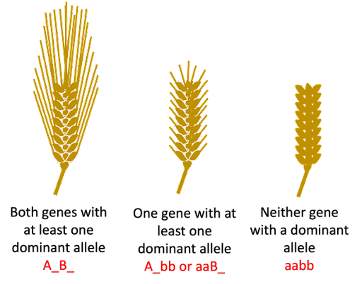
Awn length is an example of a quantitative trait: a trait that is a measurable phenotype, controlled by multiple genes acting cumulatively. We just looked at two genes, and a correspondingly limited number of phenotypes. But awn length is controlled by many more genes than just two, and there is more variation in awns than can be divided into simple phenotypic classes of long, short, and no awn.

One of the hallmarks of quantitative traits is that, rather than existing in easily distinguishable categories, the traits may vary continuously throughout a population. For comparison, you’ll recall that Mendel observed round seeds and wrinkled seeds, yellow and green seeds. Those are examples of discrete variation.

 But quantitative traits vary across a spectrum. There is no distinct separation of phenotypic classes. This is called continuous variation. One example in humans is height, which can vary from very short to very tall. Other examples of continuously variable traits in humans are skin color and weight.

Quantitative traits are controlled by multiple genes acting cumulatively. These genes are called quantitative trait loci, commonly abbreviated QTLs. The more QTLs involved, the more phenotypic classes are possible. All loci contribute additively. To make it more complicated, in many cases the alleles of these genes are incompletely dominant, so the alleles contribute additively. This gives the potential for lots of phenotypic variation with a relatively few number of genes. Let’s take a look.

You’ll recall that a monohybrid cross gives a genotypic ratio 1:2:1 (AA Aa, and aa). For incompletely dominant alleles where the heterozygote has a distinct phenotype, this gives three distinct phenotypes.

Two cumulative effect QTLs with incomplete dominance can produce five discrete phenotypes, depending on how many of the alleles associated with are present. Note that the allele symbols used here are an oversimplification: for incompletely dominant alleles where neither is dominant over the other, we would not typically use capital and lowercase letters.

• Four phenotype-associated alleles – AABB (greatest extent of phenotype)
• Three phenotype-associated alleles – AaBB or AABb
• Two phenotype-associated alleles – AAbb, AaBb, or aaBB
• One phenotype-associated allele – Aabb or aaBb
• No phenotype-associated alleles – aabb (least extent of phenotype)

Three cumulative effect QTLs with incomplete dominance can produce seven discrete phenotypes:

• Six phenotype-associated alleles – AABBCC (greatest extent of phenotype)
• Five phenotype-associated alleles – AaBBCC, AABbCC, or AABBCc
• Four phenotype-associated alleles – aaBBCC, AaBbCC, AaBBCc, AAbbCC, AABbCc, or AABBcc
• Three phenotype-associated alleles – aaBbCC, aaBBCc, AaBbCc, AabbCC, AaBBcc, AAbbCc, or AABbcc
• Two phenotype-associated alleles – AAbbcc, AaBbcc, AabbCc, aaBBcc, aaBbCc, or aabbCC
• One phenotype-associated allele – Aabbcc, aaBbcc, or aabbCc
• No phenotype-associated alleles – aabbcc (least extent of phenotype)

Four cumulative effect QTLs would produce 9 phenotypes. The relationship between the number of QTLs can be summarized with the equation below, where n = the number of loci.

# phenotypes = 2n + 1

But as the number of phenotypic classes increases, the differences between the classes get smaller. With a high enough number of genes, the discrete classes begin to blend together. This is especially true when environmental influences are factored in. For example, even identical twins who share 100% of their DNA can have slightly different heights or skin color.

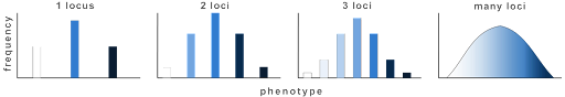
You’ll note that in all cases there are multiple genotypes that can confer an intermediate phenotype. But the most extreme phenotypes are only seen in individuals who are homozygous recessive for all alleles, or homozygous dominant. This is why, for continuously variable traits, an intermediate phenotype is the most common. Very few individuals in a population will have the most extreme phenotypes. This is illustrated in Figure 14, which shows both the number of discrete phenotypes expected for 1, 2, 3, or many QTLs and the relative frequency of each phenotype in a population^[1].

Note: this assumes that each gene contributes equally to the phenotype. In practice, however, quantitative trait loci can also vary in the extent to which they influence a trait. For example, some genes that are involved in determining height have only a modest effect, while others play a much greater role in determining height.

How many genes can affect quantitative traits? As an example in humans, there are likely hundreds of QTLs contributing to the diversity of height and hundreds of QTLs contributing to the diversity of skin color in humans.

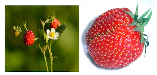
The cumulative effects of QTLs likely play a role in fruit size in polyploid commercial crops. Many of the cultivated fruits we consume, including strawberries and bananas, are much larger than their wild counterparts  . The wild counterparts are often diploid (2n = 2x). Many cultivated strawberries are octoploid (2n = 8x) and the most common cultivated bananas are triploid.

Test Your Understanding